Survival analysis in R in 15 minutes
Survival analyisis
I’ve been doing a lot of survival analysis in R recently. I use regression models all the time, but I’ve rarely had chance to use survival models, so I thought I’d write up some notes for anyone else who is getting started. These models could be considered as regressions of time-to-event data and many of the methods transfer over but survival analyses, and the Cox model in-particular, have a few quirks that differ from other cross-sectional analyses. R is set up very well for survival analysis and the survival package (Therneau, 2020) is part of the core R distribution. This post won’t be exhaustive, or an especially mathematical treatment of survival, but it will explain all you need to get started (if for example, your boss needs survival analysis urgently, possibly related to covid-19… ;-) ).
If you are interested in more depth, there are many good resources, but this post from Emily C. Zabor @zabormetrics is really nice: https://www.emilyzabor.com/tutorials/survival_analysis_in_r_tutorial.html
Set-up
As mentioned above, survival analysis is about the ‘time-to-event.’ The event is often the death of a patients/trial participant in clinical studies, so it was called “survival,” but it could be time to any sort of event. Simple survival models involve one change of state, e.g. ‘alive’ to ‘dead.’ More complicated time-to-event models allow more than one change of state (e.g. time to diagnosis of cancer, recovery after treatment, second primary cancer, treatment, end-of-life care, etc.)
We’ll use a simplified example from a group of patients who were in a heart transplant study (Crowley & Hu 1977). This is available within the survival package as the heart dataset.
We are observing patients until death (‘event’), but we don’t know anything further than the end of the study. In survival studies, patients are not necessarily in the study for the whole period. They may be recruited later than others, they may leave the study because contact is lost (‘lost to follow-up’), they may survive until the study ends or they may die. The time they leave the study without having an event (e.g. death), is the date they are ‘censored.’ Censoring can be a very complicated subject and is related to individual study contexts, but we are assuming ‘right-censored’ data where all patients have a ‘day 0’ but the end date could vary from one patient to the next. This variable survival time is added in to the study appropriately, and we get round it to some extent using the hazard function explained later.
We won’t go much more in-depth than that, but different patients have different amounts of time in the model.
Firstly, lets load the data and create a ‘survival object.’ This is a time-dependent outcome. You supply it with the survival time, or start and end dates, and a status variable that indicates the event.
library(survival)
data(heart)

dplyr::glimpse(heart)
## Rows: 172
## Columns: 8
## $ start <dbl> 0, 0, 0, 1, 0, 36, 0, 0, 0, 51, 0, 0, 0, 12, 0, 26, 0, 0, 1…
## $ stop <dbl> 50, 6, 1, 16, 36, 39, 18, 3, 51, 675, 40, 85, 12, 58, 26, 1…
## $ event <dbl> 1, 1, 0, 1, 0, 1, 1, 1, 0, 1, 1, 1, 0, 1, 0, 1, 1, 0, 1, 0,…
## $ age <dbl> -17.15537303, 3.83572895, 6.29705681, 6.29705681, -7.737166…
## $ year <dbl> 0.1232033, 0.2546201, 0.2655715, 0.2655715, 0.4900753, 0.49…
## $ surgery <dbl> 0, 0, 0, 0, 0, 0, 0, 0, 0, 0, 0, 0, 0, 0, 0, 0, 0, 0, 0, 0,…
## $ transplant <fct> 0, 0, 0, 1, 0, 1, 0, 0, 0, 1, 0, 0, 0, 1, 0, 1, 0, 0, 1, 0,…
## $ id <dbl> 1, 2, 3, 3, 4, 4, 5, 6, 7, 7, 8, 9, 10, 10, 11, 11, 12, 13,…So this looks like a start and stop time in numbered days, a status for the event, where 1 = death, patient age at start of study, the year the patient enrolled in the study, a flag for whether they have had previous bypass surgery, a flag for whether they have had a transplant, and a patient id. More details are available in the R help files: ?heart. So let’s create the survival object, called y_mortality, using the time difference from start to stop and the event indicator, and plot it (then make a nicer plot).
y_mortality <- Surv(heart$stop-heart$start, heart$event==1)

plot(y_mortality)
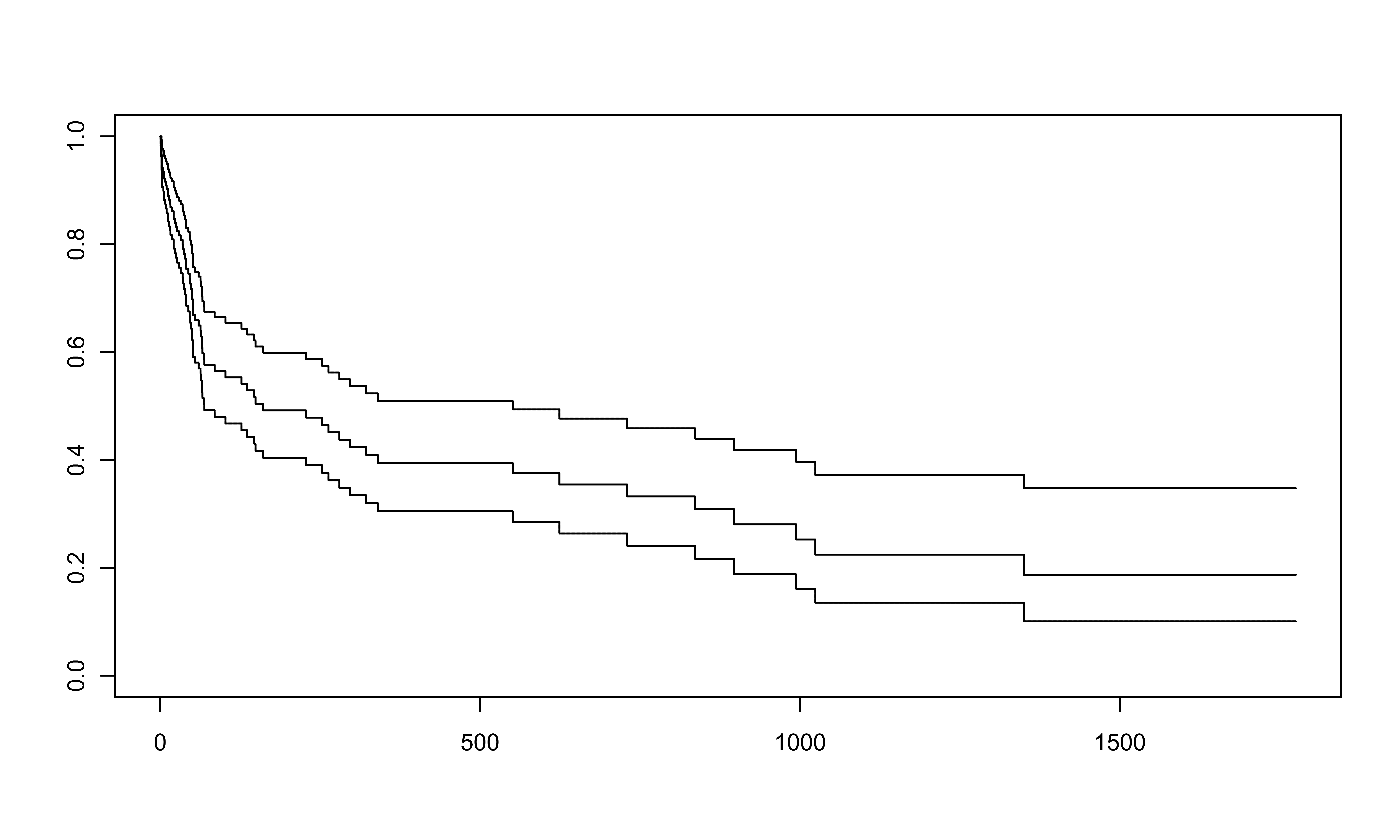
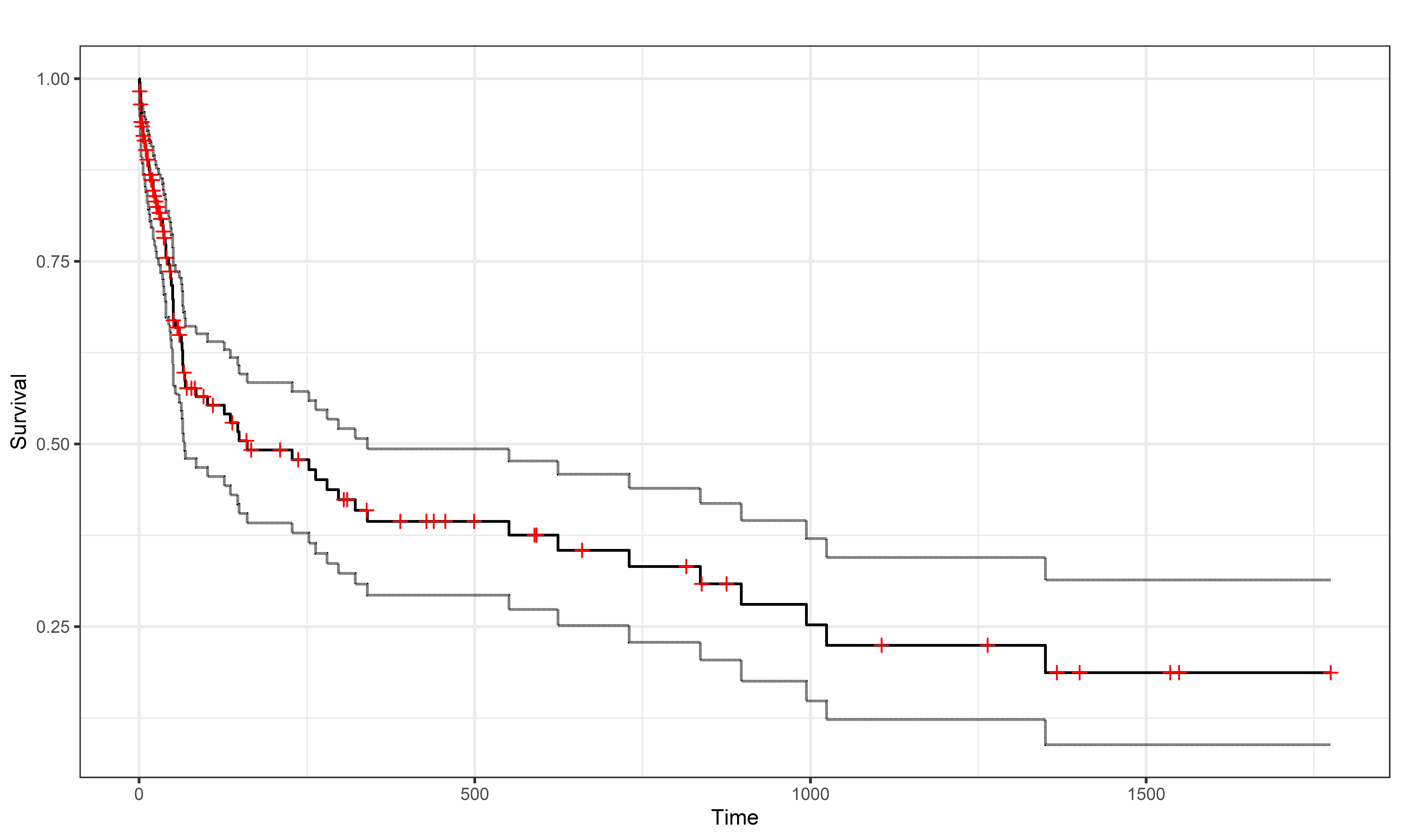
This plot is a Kaplan-Meier curve (Kaplan & Meier, 1958), and it shows the cumulative probability of the event (y-axis) at a given time (x-axis), showing the number of days in this case. Let’s make it look nicer with ggplot2, using the handy wrapper in the GGally package! The summary object is also useful as it shows us what is being plotted.
library(GGally)

surv_mortality <- survfit(y_mortality~1, conf.type="log-log")
ggsurv(surv_mortality)
summary(surv_mortality)## Call: survfit(formula = y_mortality ~ 1, conf.type = "log-log")
##
## time n.risk n.event survival std.err lower 95% CI upper 95% CI
## 0.5 172 1 0.994 0.00580 0.9595 0.999
## 1.0 171 2 0.983 0.00998 0.9469 0.994
## 2.0 166 3 0.965 0.01412 0.9233 0.984
## 3.0 160 4 0.941 0.01820 0.8925 0.968
## 5.0 150 1 0.934 0.01913 0.8847 0.963
## 6.0 147 2 0.922 0.02087 0.8689 0.954
## 8.0 144 1 0.915 0.02169 0.8611 0.949
## 9.0 141 1 0.909 0.02248 0.8532 0.944
## 10.0 140 1 0.902 0.02324 0.8454 0.939
## 12.0 136 2 0.889 0.02472 0.8295 0.929
## 14.0 129 1 0.882 0.02547 0.8213 0.923
## 15.0 128 1 0.875 0.02619 0.8131 0.918
## 16.0 127 1 0.868 0.02688 0.8050 0.912
## 18.0 123 1 0.861 0.02757 0.7967 0.907
## 21.0 119 2 0.847 0.02894 0.7798 0.895
## 23.0 114 1 0.839 0.02963 0.7711 0.889
## 25.0 112 1 0.832 0.03030 0.7624 0.883
## 26.0 110 1 0.824 0.03095 0.7537 0.876
## 29.0 103 1 0.816 0.03167 0.7444 0.870
## 32.0 98 1 0.808 0.03242 0.7347 0.863
## 35.0 94 1 0.799 0.03320 0.7247 0.856
## 36.0 93 1 0.791 0.03393 0.7147 0.849
## 37.0 90 1 0.782 0.03468 0.7046 0.841
## 39.0 86 1 0.773 0.03544 0.6941 0.834
## 40.0 85 2 0.755 0.03687 0.6734 0.819
## 44.0 81 1 0.745 0.03757 0.6628 0.811
## 46.0 80 1 0.736 0.03824 0.6524 0.803
## 47.0 77 1 0.727 0.03892 0.6416 0.795
## 48.0 76 1 0.717 0.03957 0.6310 0.786
## 50.0 75 2 0.698 0.04076 0.6099 0.770
## 51.0 73 3 0.669 0.04231 0.5788 0.744
## 54.0 68 1 0.659 0.04282 0.5682 0.736
## 60.0 65 1 0.649 0.04334 0.5572 0.727
## 63.0 63 1 0.639 0.04386 0.5461 0.718
## 64.0 62 1 0.629 0.04435 0.5351 0.708
## 65.0 61 2 0.608 0.04523 0.5132 0.690
## 66.0 59 1 0.598 0.04562 0.5024 0.681
## 68.0 56 1 0.587 0.04604 0.4912 0.671
## 69.0 55 1 0.576 0.04642 0.4801 0.661
## 85.0 50 1 0.565 0.04690 0.4679 0.651
## 102.0 48 1 0.553 0.04738 0.4555 0.640
## 127.0 46 1 0.541 0.04785 0.4428 0.629
## 136.0 45 1 0.529 0.04827 0.4303 0.618
## 147.0 43 1 0.517 0.04869 0.4175 0.607
## 149.0 42 1 0.504 0.04906 0.4049 0.596
## 161.0 40 1 0.492 0.04943 0.3919 0.584
## 228.0 37 1 0.478 0.04985 0.3782 0.572
## 253.0 35 1 0.465 0.05026 0.3641 0.559
## 263.0 34 1 0.451 0.05061 0.3502 0.547
## 280.0 33 1 0.437 0.05089 0.3365 0.534
## 297.0 32 1 0.424 0.05110 0.3229 0.521
## 322.0 29 1 0.409 0.05139 0.3082 0.507
## 340.0 27 1 0.394 0.05167 0.2931 0.493
## 551.0 21 1 0.375 0.05251 0.2735 0.477
## 624.0 18 1 0.354 0.05357 0.2515 0.459
## 730.0 16 1 0.332 0.05461 0.2286 0.439
## 836.0 14 1 0.309 0.05563 0.2043 0.419
## 897.0 11 1 0.280 0.05721 0.1754 0.395
## 994.0 10 1 0.252 0.05796 0.1483 0.371
## 1024.0 9 1 0.224 0.05791 0.1229 0.345
## 1350.0 6 1 0.187 0.05911 0.0884 0.314So by approximately 155 days, 50% of patients survived, by approximately 1000 days 25% patients survived.
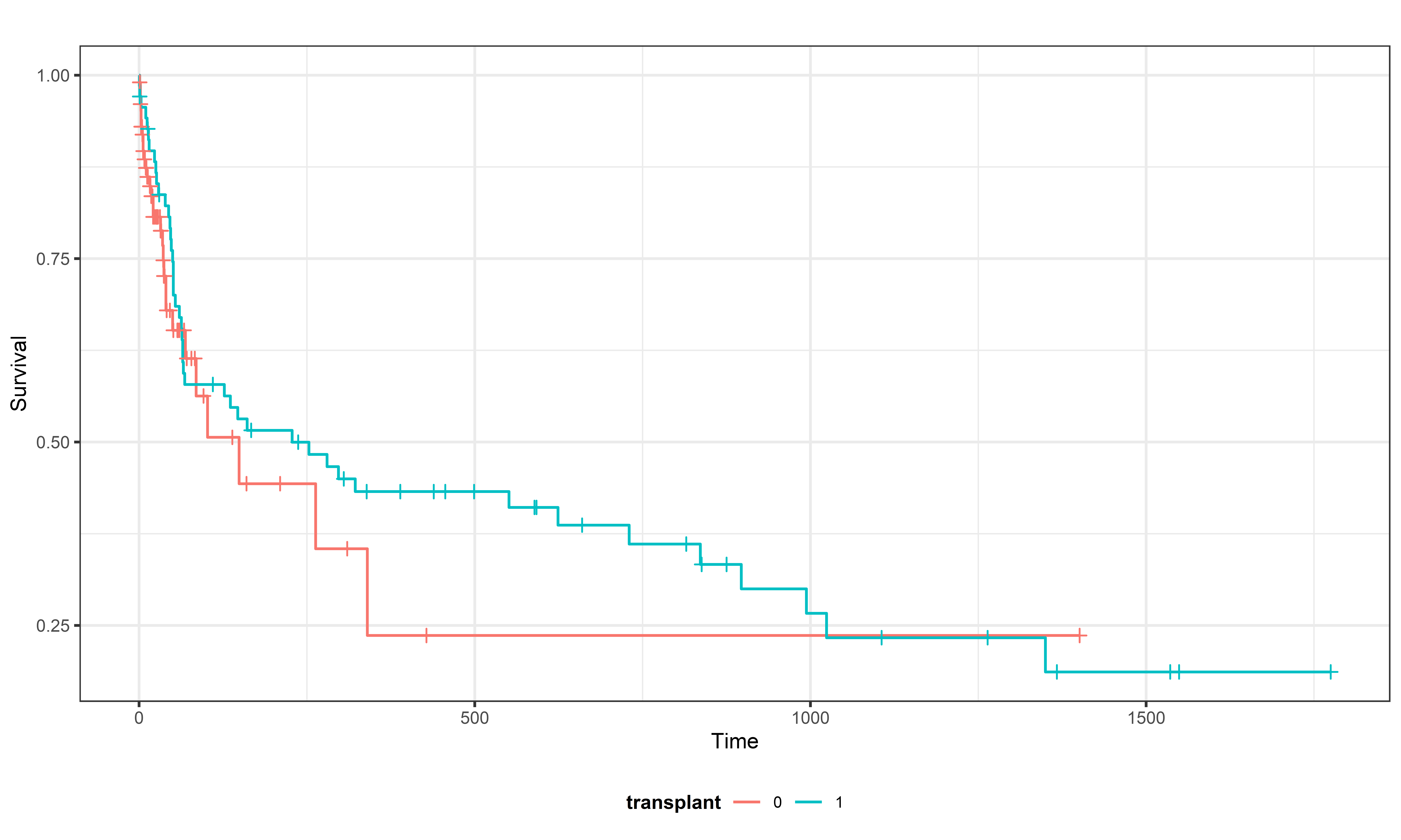
Two common ways to look at survival are to compare the plots, or to create incidence rate ratios (IRRs). we’ll use a plot below, but you can use the ratetable function for IRRs, but it required a bit more thought than a plot.
surv_mortality_transplant <- survfit(y_mortality~transplant,data=heart, conf.type="log-log")
ggsurv(surv_mortality_transplant)
So, without adjustment, it looks like patients who received transplants survive longer. There is a big ‘but’ in this interpretation though. What if only healthier patients, with better chance of survival, received transplants? This would confound the result, as these patients would be likely to survive longer anyway. What if surgical practises had changed over time, we might see some effects of this in our later patients. We need to adjust for these case-mix factors… (reaches for his trusty regression model…)
Survival regressions and risk-adjustment
Regression models are a common underlying framework for many types of analysis, and survival is no different. Here our regression also has a time dimension to it.
Hazards?
Rather than model the odds of an event as we would with logistic regression, we model the odds of event at a given time. This is commonly described as the ‘instantaneous risk of event’, or ‘instantaneous failure rate’, more formally called the hazard function. We are then modelling a ratio of the hazard function in the ‘event’ group against the ‘no-event’ group, more formally called the hazard ratio.
Cox’s proportional hazards
Professor Sir David Cox (who also proposed logistic regression amongst other things…https://en.wikipedia.org/wiki/David_Cox_(statistician) ) proposed a regression model using the hazard ratio (Cox, 1974). This allow the dependency on the event to be linked to predictors, as we would in a normal regression model, and we then have a method for casemix adjustment.
There is one key assumption of this model: ‘proportional hazards’. This means that the risk of the event doesn’t alter over the course of the study. This seems an intuitive assumption, but is commonly violated. e.g. over a long running study, the risk of death related to smoking may have changed with fewer people smoking in later years. In our recent work on covid-19 survival at UHB, we found this was violated in relation to sex. The risk of death appeared to change over the course of the study, and we theorised that is was related to length-of-stay in hospital differing by sex, but I digress…. There are mechanisms for dealing with so-called ‘time-varying’ effects, but we’ll keep it simple in this post.
For application in R we will use the Surv object we created above as our y. The KM plot showed the effects of the transplant group when looking at survival, but lets imagine that age affects the likelihood of receiving a transplant. We should adjust for age as well as transplant. So lets fit two Cox models: first one to get the estimate of the effects of transplant, and then transplant combined with effects of age:
cox_model <- coxph(y_mortality ~ transplant, data=heart)
summary(cox_model)
## Call:
## coxph(formula = y_mortality ~ transplant, data = heart)
##
## n= 172, number of events= 75
##
## coef exp(coef) se(coef) z Pr(>|z|)
## transplant1 -0.2143 0.8071 0.2541 -0.843 0.399
##
## exp(coef) exp(-coef) lower .95 upper .95
## transplant1 0.8071 1.239 0.4905 1.328
##
## Concordance= 0.534 (se = 0.031 )
## Likelihood ratio test= 0.7 on 1 df, p=0.4
## Wald test = 0.71 on 1 df, p=0.4
## Score (logrank) test = 0.71 on 1 df, p=0.4cox_model_age <- coxph(y_mortality ~ age + transplant, data=heart)
summary(cox_model_age)## Call:
## coxph(formula = y_mortality ~ age + transplant, data = heart)
##
## n= 172, number of events= 75
##
## coef exp(coef) se(coef) z Pr(>|z|)
## age 0.03236 1.03289 0.01473 2.197 0.028 *
## transplant1 -0.32182 0.72483 0.26108 -1.233 0.218
## ---
## Signif. codes: 0 '***' 0.001 '**' 0.01 '*' 0.05 '.' 0.1 ' ' 1
##
## exp(coef) exp(-coef) lower .95 upper .95
## age 1.0329 0.9682 1.0035 1.063
## transplant1 0.7248 1.3796 0.4345 1.209
##
## Concordance= 0.595 (se = 0.04 )
## Likelihood ratio test= 6.09 on 2 df, p=0.05
## Wald test = 5.62 on 2 df, p=0.06
## Score (logrank) test = 5.65 on 2 df, p=0.06The output above suggests that receiving transplant doesn’t significantly affect risk of death (if we blindly use the 95% threshold that we often do…). When we add in age, it is still not significant, but it’s affects are stronger once we remove the confounding of age. We could also check with an interaction term, but I don’t think it’s logical. My suspicion is that older patients are less likely to receive transplanted organs, rather that the effects of a transplant being different with age. (I did check it just in-case but no improvement in AIC, explained later…).
The help files say that the age columns is: age - 48 years. This suggests that 48 years was the average age, and they have mean-centred the age. This is a useful tool, as it allows you to read the coefficient as the risk for the ‘average’ patient. Here though, the important part to note is that increasing age slightly increases the hazard ratio, or risk of death, whereas transplant reduces it, but it is not ‘statistically significant.’
Now, let’s go all in…
cox_model_all <- coxph(y_mortality ~ age + transplant + surgery + year, data=heart)
summary(cox_model_all)
## Call:
## coxph(formula = y_mortality ~ age + transplant + surgery + year,
## data = heart)
##
## n= 172, number of events= 75
##
## coef exp(coef) se(coef) z Pr(>|z|)
## age 0.02819 1.02859 0.01386 2.034 0.0419 *
## transplant1 -0.28292 0.75358 0.26314 -1.075 0.2823
## surgery -0.66423 0.51467 0.36634 -1.813 0.0698 .
## year -0.15234 0.85870 0.07056 -2.159 0.0309 *
## ---
## Signif. codes: 0 '***' 0.001 '**' 0.01 '*' 0.05 '.' 0.1 ' ' 1
##
## exp(coef) exp(-coef) lower .95 upper .95
## age 1.0286 0.9722 1.0010 1.0569
## transplant1 0.7536 1.3270 0.4499 1.2622
## surgery 0.5147 1.9430 0.2510 1.0553
## year 0.8587 1.1646 0.7478 0.9861
##
## Concordance= 0.648 (se = 0.034 )
## Likelihood ratio test= 16.85 on 4 df, p=0.002
## Wald test = 15.98 on 4 df, p=0.003
## Score (logrank) test = 16.62 on 4 df, p=0.002So, that’s interesting. ‘surgery,’ (having received prior bypass surgery) significantly reduces the risk of death, as does ‘year’ (year patient entered the study, number in years from Nov 1967). This suggest that survival has improved over years, and prior bypass surgery is protective. This may be a surrogate indicator of a ‘stronger’ patient, who would have been assessed as strong enough for surgery.
How do we tell which model is better?
As with many things in stats, there are various ways and each has it’s pros and cons. I like to use the Akaike Information Criterion (AIC) (Akaike, 1998). This is a relative value which represents the amount of information lost, with smaller values (closer to zero) suggesting less information is lost. It is approximately \(\chi ^2\) distributed on one degree-of-freedom, and essentially means a change of 4 in the AIC is significant at 95%. For more information on AIC, I’d recommend Burnham & Anderson (2004) and Greven & Kneib (2010).
AIC(cox_model)## [1] 634.7102AIC(cox_model_age)## [1] 631.3196AIC(cox_model_all)## [1] 624.56The AIC of our full model is much lower here, so it’s a ‘better’ model that loses less information.
Summary
This post has taken a brief tour of survival analysis in R. This is about the time to event, and that event was originally (and often is) death in a clinical study. We can use this information to visualise survival using Kaplan-Meier curves, and use the tools in our regression tool box when we use a proportional hazards model, commonly called ‘Cox’ model, named after it’s creator.
This is just the surface of survival analyses in R, and the survival package by Terry Therneau is a powerhouse, with a fantastic set of vignette examples covering so much theory and application. There is much more to this field, including time-varying predictors, multi-state models, landmark analysis etc. I hope this post can get you started, clear the fog around using survival analyses, and allow you to learn more from vignettes, tutorials and literature.
References
AKAIKE, H. 1998. Information Theory and an Extension of the Maximum Likelihood Principle. In: PARZEN, E., TANABE, K. & KITAGAWA, G. (eds.) Selected Papers of Hirotugu Akaike. New York, NY: Springer New York.
BURNHAM, K. P. & ANDERSON, D. R. 2004. Multimodel Inference: Understanding AIC and BIC in Model Selection. Sociological Methods & Research, 33, 261-304.
COX, D. R. 1972. Regression Models and Life-Tables. Journal of the Royal Statistical Society, Series B. 34 (2): 187–220. JSTOR 2985181. MR 0341758.
COX, D.R., OAKES, D., 1984. Analysis of Survival Data, Chapman & Hall/CRC Monographs on Statistics & Applied Probability. Taylor & Francis.
CROWLEY, J., HU, M., 1977, Covariance analysis of heart transplant survival data. Journal of the American Statistical Association, 72, 27–36.
GREVEN, S. & KNEIB, T. 2010. On the behaviour of marginal and conditional AIC in linear mixed models. Biometrika, 97, 773-789.
KAPLAN, E. L. & MEIER, P. (1958). Nonparametric estimation from incomplete observations. J. Amer. Statist. Assoc. 53 (282): 457–481. doi:10.2307/2281868. JSTOR 2281868.
THERNEAU, T., 2020. A Package for Survival Analysis in R. R package version 3.1-12, <URL: https://CRAN.R-project.org/package=survival>.
THERNEAU, T.M., GRAMBSCH, P.M, 2000. Modeling Survival Data: Extending the Cox Model. Springer, New York. ISBN 0-387-98784-3.